Getting started with classifiers
Classifiers are supervised neural networks that can be trained to automatically predict the class label of a data sample based on it spectral characteristics. Classifiers are trained to map input data samples to one-hot binary vectors which indicate the class of the data sample. The network requires data samples with class labels to train on (hence it is supervised). Once trained, a classifier can predict the class of new data samples.
Download a hyperspectral dataset
Some hyperspectral datasets in a matlab file format (.mat) can be downloaded from here. To get started, download the ‘Pavia University’ dataset and its ground truth labels.
deephyp operates on hyperspectral data in numpy array format. The matlab files (.mat) you just downloaded can be read as a numpy array using the scipy.io.loadmat function:
import scipy.io
mat = scipy.io.loadmat( 'PaviaU.mat' )
img = mat[ 'paviaU' ]
where img is a numpy array. Use the same function to read the ground truth class labels:
mat_gt = scipy.io.loadmat('PaviaU_gt.mat')
img_gt = mat_gt['paviaU_gt']
You are now ready to use the toolbox!
Overview
For both autoencoders and classifiers, the toolbox uses several key processes:
- data preparation
- data iterator
- building networks
- adding train operations
- training networks
- loading and testing a trained network
Each of these are elaborated on below:
Data preparation
A class within the toolbox from the data module called HypImg handles the hyperspectral dataset and all of its meta-data. As mentioned earlier, the class accepts the hyperspectral data in numpy format, with shape [numRows x numCols x numBands] or [numSamples x numBands]. The networks in the toolbox operate in the spectral domain, not the spatial, so if a hypercube image is input with shape [numRows x numCols x numBands], it is reshaped to [numSamples x numBands], collapsing the spatial dimensions into a single dimension.
The Pavia Uni hyperspectral image and labels can be passed to the HypImg class as follows:
from deephyp import data
hypData = data.HypImg( img, labels=img_gt )
Upon initialisation the HypImg object will automatically generate one-hot labels from the labels input, stored in the labelsOnehot attribute. Classes with a label <= 0 are considered a background class, and are not included in the numClasses attribute. Any samples with a zero label will appear as a row of zeros in labelsOnehot.
The data can be pre-processed using a function of the HypImg class. For example, using the ‘minmax’ approach:
hypData.pre_process( 'minmax' )
The result is stored in the spectraPrep attribute. Currently, only the ‘minmax’ approach is available, but additions will be made in future versions.
Data iterator
The Iterator class within the data module has methods for calling batches from the data that are used to train the network. A separate iterator object is made for the training and validation data.
Before setting up an Iterator object, establish which data samples from the hyperspectral image you will use to train and validate the network. For example, you can use the following code to get the indexes of 50 training samples and 15 validation samples per class, for each of the nine non-background classes in the Pavia Uni dataset:
import numpy as np
trainSamples = 50 # per class
valSamples = 15 # per class
train_indexes = []
for i in range(1,10):
    train_indexes += np.nonzero(hypData.labels == i)[0][:trainSamples].tolist()
val_indexes = []
for i in range(1,10):
    val_indexes += np.nonzero(hypData.labels == i)[0][trainSamples:trainSamples+valSamples].tolist()
Now, to build an iterator object for training from the pre-processed hyperspectral training samples and their labels, with a batchsize of 50, use:
dataTrain = data.Iterator( dataSamples=hypData.spectraPrep[train_indexes, :], targets=hypData.labelsOnehot[train_indexes,:], batchSize=50 )
Since we are training a supervised classifier, the targets are the ground truth class labels.
Similarly, an iterator object for validation is defined with:
dataVal = data.Iterator( dataSamples=hypData.spectraPrep[val_indexes, :], targets=hypData.labelsOnehot[val_indexes,:] )
Because the batchsize is unspecified for the validation iterator, all samples are used for each batch.
The data in any iterator can also be shuffled before it is used to train a network:
dataTrain.shuffle()
Building networks
The classifier module has a class for creating supervised classification neural networks:
from deephyp import classifier
There is currently one type of classifier that can be set up, which contains a combination of convolutional layers (at the start) and fully-connected layers (at the end).:
net = classifier.cnn_1D_network( inputSize=hypData.numBands, numClasses=hypData.numClasses )
If not using config files to set up a network, then the input size of the data (which should be the number of spectral bands) and the number of classes must be specified. These are stored in hypData.numBands and hypData.numClasses for convenience.
Additional aspects of the network architecture can also be specified when initialising the classifier object:
net = classifier.cnn_1D_network( inputSize=hypData.numBands, numClasses=hypData.numClasses, convFilterSize=[20,10,10], convNumFilters=[10,10,10], convStride = [1,1,1], fcSize=[20,20], activationFunc='relu', weightInitOpt='truncated_normal', padding='VALID' )
where the following components of the architecture can be specified:
- number of convolutional layers - this is the length of the list ‘convNumFilters’
- number of filters/kernels in each conv layer - these are the values in the ‘convNumFilters’ list
- the size of the filters/kernels in each conv layer - these are the values in the ‘convFilterSize’ list
- the stride of the filters/kernels in each conv layer - these are the values in the ‘convStride’ list
- the type of padding each conv layer uses - padding
- number of fully-connected layers - this is the length of the list ‘fcSize’
- number of neurons in each fully-connected layer - these are the values in the ‘fcSize’ list
- the activation function which proceeds each layer - activationFunc
- the method of initialising network parameters (e.g. xavier improved) - ‘weightInitOpt’
Therefore, the above CNN classifier has three convolutional layers, two fully-connected layers and an output layer. The three convolutional layers each have 10 filters, with sizes 20, 10 and 10. The fully-connected layers both have 20 neurons.
Instead of defining the network architecture by the initialisation arguments, a config.json file can be used:
net = classifier.cnn_1D_network( configFile='config.json') )
A config file is generated each time a network in the toolbox is trained, so you can use one from another network as a template for making a new one.
Adding training operations
Once a network has been created, a training operation can be added to it. It is possible to add multiple training operations to a network, so each op must be given a name:
net.add_train_op( name='experiment_1' )
When adding a train op, details about how the network will be trained with that op can also be specified. For example, a train op for a classifier with a learning rate of 0.001 with no decay, optimised with Adam, class balancing and no weight decay can be defined by:
net.add_train_op( name='experiment_1', balance_classes=True, learning_rate=1e-3, method='Adam', wd_lambda=0.0 )
Classification networks are trained using a cross-entropy loss function.
The method for decaying the learning rate can also be customised. For example, to decay the learning rate exponentially every 100 steps (starting at 0.001):
net.add_train_op( name='experiment_1',learning_rate=1e-3, decay_steps=100, decay_rate=0.9 )
A piecewise approach to decaying the learning rate can also be used. For example, to change the learning rate from 0.001 to 0.0001 after 100 steps, and then to 0.00001 after a further 200 steps:
net.add_train_op( name='experiment_1',learning_rate=1e-3, piecewise_bounds=[100,300], piecewise_values=[1e-4,1e-5] )
Training networks
Once one or multiple training ops have been added to a network, they can be used to learn a model (or multiple models) for that network through training:
net.train( dataTrain=dataTrain, dataVal=dataVal, train_op_name='experiment_1', n_epochs=100, save_addr=model_directory, visualiseRateTrain=5, visualiseRateVal=10, save_epochs=[50,100])
The train method learns a model using one train op, therefore the train method should be called at least once for each train op that was added. The name of the train op must be specified, and the training and validation iterators created previously must be input. A path to a directory to save the model must also be specified. The example above will train a network for 100 epochs of the training dataset (that is, loop through the entire training dataset 100 times), and save the model at 50 and 100 epochs. The training loss will be displayed every 5 epochs, and the validation loss will be displayed every 10 epochs.
It is also possible to load a pre-trained model and continue to train it by passing the address of the epoch folder containing the model checkpoint as the save_addr argument. For example, if the directory for the model at epoch 50 (epoch_50 folder) was passed to save_addr in the example above, then the model would initialise with the epoch 50 parameters and be trained for an additional 50 epochs to reach 100, at which point the model would be saved in a folder called epoch_100 in the same directory as the epoch_50 folder.
The interface for training autoencoders and classifiers is the same.
Loading and testing a trained network
Once you have a trained network, it can be loaded and tested out on some hyperspectral data.
Open a new python script. To load a trained model on a new dataset, ensure the data has been pre-processed similarly using:
from deephyp import data
new_hypData = data.HypImg( new_img )
new_hypData.pre_process( 'minmax' )
When doing inference, labels do not need to be input into HypImg (unless you want to use them for evaluation).
Set up the network. The network architecture must be the same as the one used to train the model being loaded. However, this is easy as the directory where models are saved should contain an automatically generated config.json file, which can be used to set up the network with the same architecture:
from deephyp import classifier
net = classifier.cnn_1D_network( configFile='model_directory/config.json' )
Once the architecture has been defined, add a model to the network. For example, adding the model that was saved at epoch 100:
net.add_model( addr='model_directory/epoch_100'), modelName='clf_100' )
Because multiple models can be added to a single network, the added model must be given a name. The name can be anything - the above model is named ‘clf_100’ because it is a classifier and was trained for 100 epochs).
When the network is set up and a model has been added, hyperspectral data can be passed through it. To use a trained classifier to predict the classification labels of some spectra:
dataPred = net.predict_labels( modelName='clf_100', dataSamples=new_hypData.spectraPrep )
Like-wise, to predict the classification scores for each class of some spectra:
dataScores = net.predict_scores( modelName='clf_100', dataSamples=new_hypData.spectraPrep )
To extract the features in the second last layer of the classifier network:
dataFeatures = net.predict_features( modelName='clf_100', dataSamples=new_hypData.spectraPrep, layer=net.numLayers-1 )
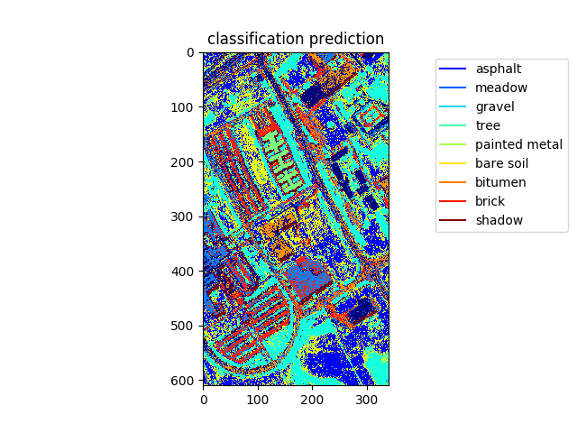
You can use numpy to reshape the predicted labels (dataPred) so that they look like an image again:
imgPred = numpy.reshape( dataPred, ( new_hypData.numRows, new_hypData.numCols ) )
Now you should have a basic idea of how to use the deephyp toolbox to train a classifier for hyperspectral data!